Import the fashion MNIST dataset
Code
import tensorflow as tfimport pandas as pdimport numpy as npimport matplotlib.pyplot as pltprint (tf.__version__)= tf.keras.datasets.fashion_mnist= fashion_data.load_data()
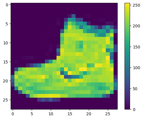
Preprocessing the data
Code
0 ])False )
Code
= train_data[:5000 ] / 255.0 , train_data[5000 :]/ 255.0 = train_label[:5000 ], train_label[5000 :]
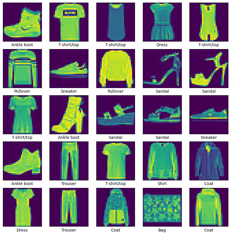
Code
= ['T-shirt/top' , 'Trouser' , 'Pullover' , 'Dress' , 'Coat' ,'Sandal' , 'Shirt' , 'Sneaker' , 'Bag' , 'Ankle boot' ]
Code
= (10 ,10 ))for i in range (25 ):5 ,5 , i+ 1 )
Building the model using neural network
Sequential Model is the simplest form of Model that keras library provides. It is composed of a single stack of layer connected sequentially. Also, known as sequential API. The first layer in the model is is Flatten model ,which simply flattens the 2D image array to 1D. Then, the Dense layer with 300 neurons which uses Relu as an activation function is stacked. Then, there is second Dense layer with 100 neurons , with same Relu as activation function. The final layer in the model stack is output layuer, which is also a Dense layer with 10 neurons (one per class) and it uses softmax function for multi-class classification.
Code
= tf.keras.layers.Flatten(input_shape= (28 ,28 ))= tf.keras.layers.Dense(300 , activation= 'relu' )= tf.keras.layers.Dense(100 , activation= 'relu' )= tf.keras.layers.Dense(10 , activation = 'softmax' )= tf.keras.Sequential([input_layer,dense_layer1, dense_layer2 ,output_layer])= 'adam' = tf.keras.losses.SparseCategoricalCrossentropy()= ['accuracy' ]
Model: "sequential"
_________________________________________________________________
 Layer (type)                Output Shape              Param #
=================================================================
 flatten (Flatten)           (None, 784)               0

 dense (Dense)               (None, 300)               235500

 dense_1 (Dense)             (None, 100)               30100

 dense_2 (Dense)             (None, 10)                1010

=================================================================
Total params: 266610 (1.02 MB)
Trainable params: 266610 (1.02 MB)
Non-trainable params: 0 (0.00 Byte)
_________________________________________________________________
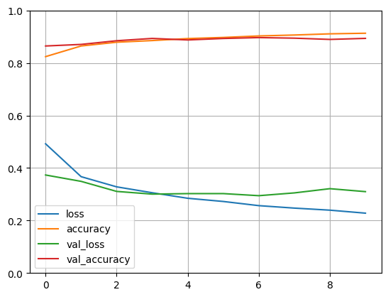
Training the model
Code
compile (optimizer= optimizer, loss= loss_function, metrics= metrics )= model.fit(x_train,y_train, epochs= 10 , validation_data = (x_valid, y_valid))
Epoch 1/10
1719/1719 [==============================] - 2s 852us/step - loss: 0.4921 - accuracy: 0.8241 - val_loss: 0.3733 - val_accuracy: 0.8646
Epoch 2/10
1719/1719 [==============================] - 1s 788us/step - loss: 0.3670 - accuracy: 0.8647 - val_loss: 0.3491 - val_accuracy: 0.8706
Epoch 3/10
1719/1719 [==============================] - 2s 891us/step - loss: 0.3282 - accuracy: 0.8789 - val_loss: 0.3108 - val_accuracy: 0.8846
Epoch 4/10
1719/1719 [==============================] - 1s 775us/step - loss: 0.3058 - accuracy: 0.8853 - val_loss: 0.3005 - val_accuracy: 0.8934
Epoch 5/10
1719/1719 [==============================] - 1s 822us/step - loss: 0.2847 - accuracy: 0.8929 - val_loss: 0.3024 - val_accuracy: 0.8876
Epoch 6/10
1719/1719 [==============================] - 1s 769us/step - loss: 0.2725 - accuracy: 0.8971 - val_loss: 0.3025 - val_accuracy: 0.8932
Epoch 7/10
1719/1719 [==============================] - 1s 799us/step - loss: 0.2566 - accuracy: 0.9029 - val_loss: 0.2946 - val_accuracy: 0.8966
Epoch 8/10
1719/1719 [==============================] - 1s 776us/step - loss: 0.2473 - accuracy: 0.9064 - val_loss: 0.3052 - val_accuracy: 0.8944
Epoch 9/10
1719/1719 [==============================] - 1s 784us/step - loss: 0.2394 - accuracy: 0.9109 - val_loss: 0.3212 - val_accuracy: 0.8896
Epoch 10/10
1719/1719 [==============================] - 1s 818us/step - loss: 0.2280 - accuracy: 0.9131 - val_loss: 0.3100 - val_accuracy: 0.8936
Code
True )0 ,1 )
Testing the model
Code
= model.evaluate(test_data, test_label)
313/313 [==============================] - 0s 433us/step - loss: 55.4865 - accuracy: 0.8696